Finding Colours - Part 2: Maths is hard

Ok in part 1 we looked at finding dominant colours in an image, we got as far as showing the top 8 colours by pixel count, and showed that this isn't necessarily the best solution for real-world images as there are micro variations of colour within the image that aren't always immediately obvious to the naked eye.

Let's take a closer look at the first image we had trouble with the Panda:

The original image is cropped from a 10-megapixel DSLR and looks reasonably sharp but let's see what it looks like if we zoom in to the point where the individual pixels become visible:

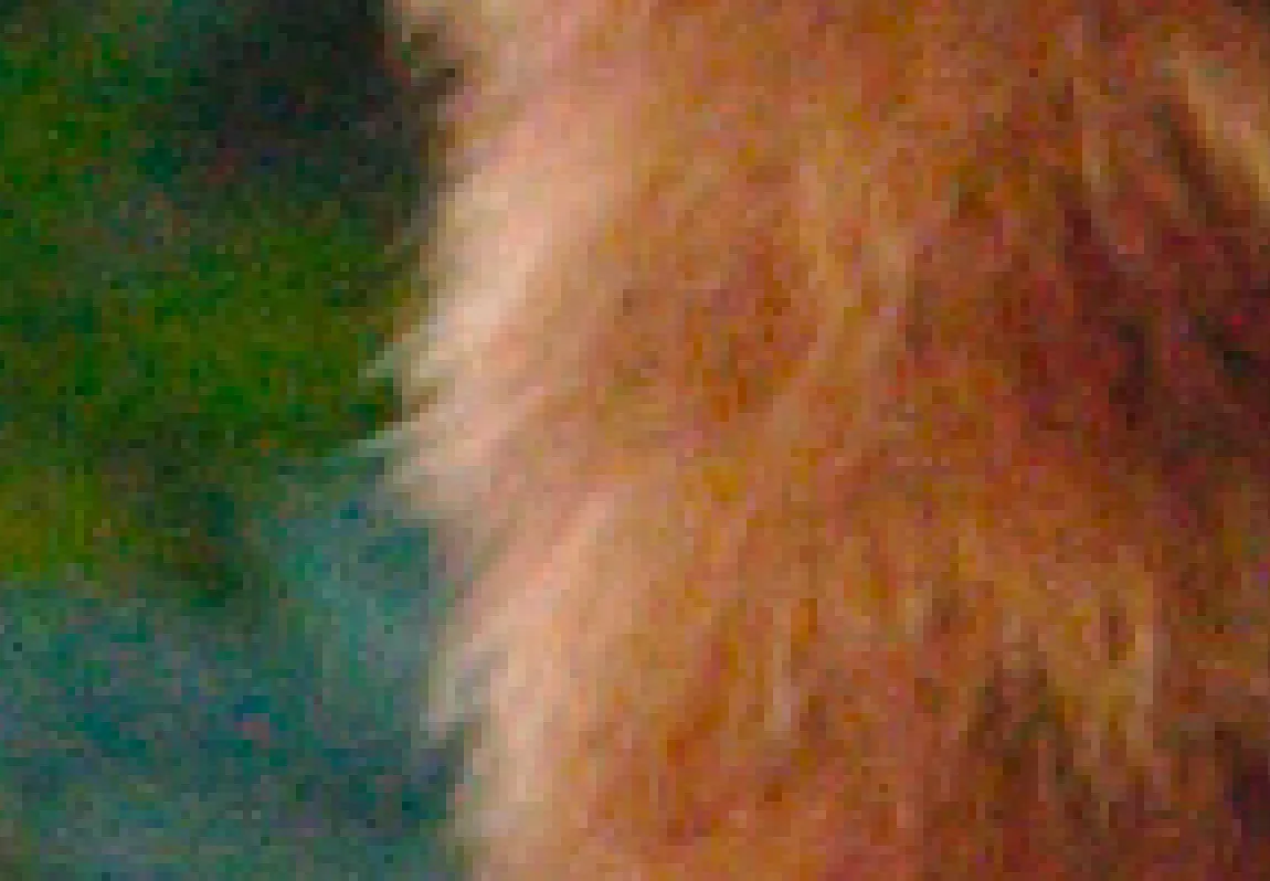
At around 400% we can see that there's a fair amount of noise in this image, and what looks like single blocks of colour to our eyes are actually made up of many small colour variations that blend together into what we see.

So how do we go from this to pulling out what we could consider dominant colours from the image? Let's take a look at one potential way of doing things.

k-means clustering

We're looking to find distinct groups of similar colours, to do this we'll use what's known as k-means clustering we're going to use the naïve k-means which is one of the more simple versions of the algorithm and is unoptimized. The basic steps are as follows:

1. Grab all of the colours from the image as 3-point coordinates

2. Determine an initial set of points, we'll select these at random, our k clusters

3. Assign each colour to one of these initial k means based on the colours' Euclidean distance to the cluster

4. Update the means centroids based on the colours assigned to it

We repeat steps 3 and 4 until updates no longer change the k-means, this is known as convergence

It should be noted that the algorithm may never actually converge, so we'll probably add in an artificial limit to how many times we want to run our assign/update steps.

Colours in 3D space

Let's revisit our ImageData from the previous post. This contains a representation of the image split as a UInt8ClampedArray which might look something like the following:

     pixel 1         pixel 2         pixel 3         pixel 4
|---------------|---------------|---------------|---------------|
|255|255|255|255| 0 | 0 | 0 |255|255|255|255|255| 0 | 0 | 0 |255|
|---------------|---------------|---------------|---------------|
    #FFFFFFFF       #000000FF       #FFFFFFFF       #000000FF

So each pixel here is made up of 3 colours that can be represented as an integer between 0 and 255 (we're ignoring the alpha channel which deals with the pixels' opacity).

Let's imagine these colours as a point in 3-dimensional space, where our red, green, and blue values become (x, y, z) coordinates, so a fully black pixel would exist at the origin (0, 0, 0) and a white one would be at the point (255, 255, 255).

Let's change up the code to give us an array of unique colour objects in the form { r: number, b: number, g: number }, we'll remove most of the code in our file, everything after we grab the imageData array:

const imageData = ctx.getImageData(0, 0, ibm.width, ibm.height).data;

let colorData = [];

for (i = 0; i < imageData.length; i += 4) {
	const colStr = [
		imageData[i],
		imageData[i+1],
		imageData[i+2]
	].join(',');

	colorData.push(colStr);
}

// 1
colorData = [...new Set(colorData)];

colorData = colorData.map(v => {
	const rgb = v.split(',');
	return {
		r: rgb[0],
		g: rgb[1],
		b: rgb[2],
	};
});

So we initially now create a string of the colour with each channel separated by a comma. The reason behind this is it makes it super simple (and quick) to reduce this to unique colours by simply pushing the array into a Set and spreading this back into an array (1), after that, we map these strings back into objects and we're done.

If we take the cropped section of our panda image above it would create a set of colours that will look as follows when graphed:

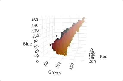
The generation of these graphs is a little outside the scope of this post so I'll not be going over it just the creation of the dataset because that's what we'll be using for our colour calculations. If you want to know more check out the project's source and the Plotly.js library

Random k-clusters

For the next step we'll take 8 unique random colours from our array using the following:

let kClusters = Array.from({ length: 8 }, () => {
	return colorData[
		Math.floor(Math.random() * colorData.length)
	];
});

Array.from lets us provide a set of config options to define the length of the array we want and a mapping function that we can use to populate the array with random items from our colorData array. There is a slight chance here that we could have duplicated initial clusters but this should be low enough to not be a problem on most images with a reasonably high enough number of distinct colours.

Assign colours to clusters

Now we have our initial clusters we're going to assign every colour to one (and just one) of these clusters. Remember we started treating colours as points in 3D space? Well, this is why for each point we will calculate what's known as the Euclidean distance to each of our k-clusters and assign the colour to the closest one.

The equation to calculate this is the following for points p,q.

What we're doing in the above is repeatedly applying the Pythagorean theorem for each of our 3 planes as shown in the image below:

First, we'll add a function to calculate this distance outside of our drop handler:

function calcEuclideanDist(p, q) {
	return Math.sqrt(
		Math.pow(p.r - q.r, 2) +
		Math.pow(p.g - q.g, 2) +
		Math.pow(p.b - q.b, 2)
	);
}

Built-in Math functions can be used here so no big calculations are needed from us.

Now we need to assign all of our unique colours to one of the selected k-clusters. For the first attempt at this, we'll run a reducer over the colorData array we created earlier:

// 1
const clusteredData = colorData.reduce(
	(prev, curr) => {
		// 2
		const distances = kClusters.map((k) => calcEuclideanDist(k, curr));
		// 3
		const minDistance = distances.reduce(
			(a, b) => Math.min(a, b),
			Infinity
		);
		// 4
		const selectedK = distances.findIndex((e) => e === minDistance);

		// 5
		prev[selectedK] = [...prev[selectedK], curr];

		return prev;
	},
	Array.from({ length: 8 }, () => [])
);

I say the first attempt because this reducer is pretty inefficient, for our zoomed image with ~125k unique colours it took around 25s to complete and since we'll be running this in multiple passes per image that time will add up significantly. We'll leave optimisation for now though and go through this line by line:

1. we create our reducer function for our colorData array and create a 2D array as our initial value.

2. we map the kClusters array and call our calcEuclideanDist function passing the current cluster and colour

3. another reducer then to find the smallest distance from our newly created distances array. We could just spread the array into Math.min here but that will fail if we ever decide to increase the number of k-clusters beyond a certain point

4. now we know the smallest distance we get its index from distances

5. and now add this colour to the array at that index in the array we are creating in this reducer. Phew

What we've created here in our clusteredData is an 8-item array with all our image colours sorted into the same index as our initially created clusters. If we console log it out it'll look something like this:

(8) [Array(24865), Array(32390), Array(7014), Array(3894), 
Array(3236), Array(19094), Array(18360), Array(16286)]

Update our k-clusters

Now we have all of our colour points assigned to one of the clusters we'll use these collections to recalculate what our k-clusters should be. The formula to do this is as follows:

This looks complicated but it's really just telling us that for each of the coordinate components (x,y,z), or in our case (r,g,b), for all of the colours in our cluster array, we take the average of that component and use it... I think.

We can calculate these new clusters by mapping over our clustered data and averaging the individual channel components:

const newKs = clusteredData.map((colors) => {
	let r = 0;
	let g = 0;
	let b = 0;

	colors.forEach((color) => {
		r += color.r;
		g += color.g;
		b += color.b;
	});

	return {
		r: Math.round(r / colors.length),
		g: Math.round(g / colors.length),
		b: Math.round(b / colors.length),
	};
});

Iterating to find clusters

Ok, we're not quite done yet. We need a way to iterate over this process and a way of determining whether or not we're 'done'.

As mentioned before given the nature of the algorithm and the fact that we're rounding values in certain places there is a chance that it will never fully converge, that is, our k-clusters will never stop updating their positions on subsequent iterations.

I'm going to take 2 approaches to solve this issue, the first will simply be a hard limit on the number of iterations allowed, say 10, and the second will be to calculate the distance shifted between our old and new clusters and stop if this shift falls below a certain threshold.

First off let's move our two cluster calculation steps from above out into their own function

function calcNewClusters(kClusters, colorData) {
	const clusteredData = colorData.reduce(
		// ...
	);

	const newKs = clusteredData.map((colors) => {
		// ...
	});

	return newKs;
}

Where this code used to be, after the initialisation of our initial k-clusters, we'll create 3 new variables

let iterations = 0;
let distanceShift = 0;
let newClusters = [];

iterations will hold how many times we've run through our steps, we'll use this to enforce our hard limit, distanceShift will be used to hold the change between the newly calculated set of k-clusters newClusters and the previous one.

I'm going to use a do/while loop here to call our calcNewClusters function, calculate our distanceShift, and replace our current set of k-clusters with the newly generated one.

do {
	newClusters = calcNewClusters(kClusters, colorData);

	newClusters.forEach((v, i) => {
		distanceShift += calcEuclideanDist(v, kClusters[i]);
	});

	distanceShift = distanceShift / newClusters.length;

	kClusters = newClusters;
	iterations += 1;
} while (distanceShift >= 5 && iterations < 10);

For distanceShift once we've found our new clusters, we take each of those and calculate the Euclidean distance between it and its previous position and average these distances. I've arbitrarily chosen 5 to be the minimum required shift before we consider our iterations done but you can try other values here if you like.

Update swatches

The final step then is to update our swatches to use our found k-clusters:

for (i = 0; i < kClusters.length; i++) {
	let swatch = document.createElement("span");
	const colorStr = `#${kClusters[i].r
		.toString(16)
		.padStart(2, "0")}${kClusters[i].g
		.toString(16)
		.padStart(2, "0")}${kClusters[i].b
		.toString(16)
		.padStart(2, "0")}`;

	const color = document.createTextNode(colorStr);
	swatch.appendChild(color);
	swatch.classList.add("p-2");
	swatch.classList.add("mb-2");
	swatch.style.backgroundColor = colorStr;

	swatches.appendChild(swatch);
}

The only difference here is we're generating a hex string from our colour objects.

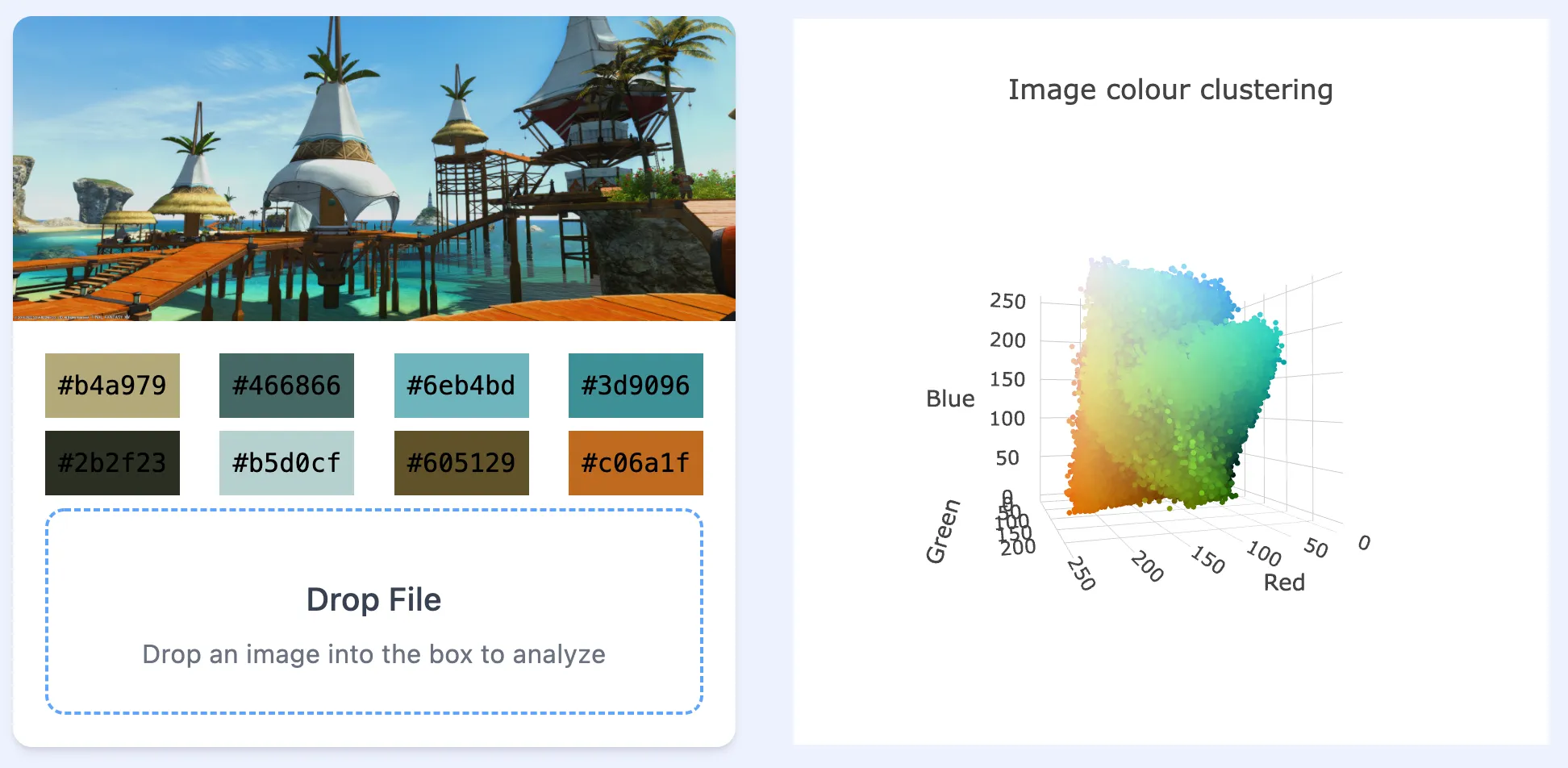
And this looks a lot better, there will always be some level of randomness in what the eventual clusters chosen might be because of the calculations, but this is a lot better than what we had before.

So this time we're done, right?

Well, no. As mentioned earlier this code has some serious efficiency problems, the image above was about 1000x400 pixels and this calculation took 5 iterations (the distanceShift went down to 3.5), but this took over 80 seconds!

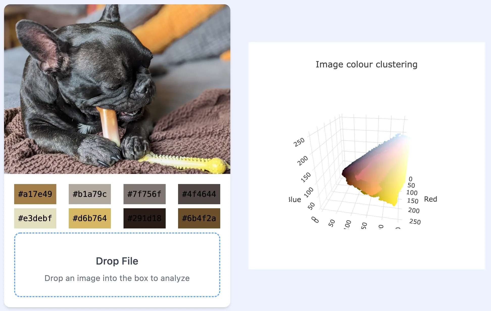
This shows some of the other drawbacks, the colours here look good but I would expect to see some deeper oranges, the brighter yellow, or even something closer to black. This is likely due to the random nature of the initial choice of clusters. Also, it took over 5 minutes for 6 iterations on this 4000x3000 pixel image.

We'll look at addressing these issues in Part 3 of this series. For now, though, the completed code for this part can be found in our GitHub repository